
Demand forecasting is the task of projecting the future demand of a firm. The demand forecast indicates how much of a product is likely to be sold during a specified future period in a specified market, at specified prices.
Demand forecasting serves as the starting point for practically each and every activity. It enables the firm to identify its precise position in. the market; this, in turn, facilitates optimum utilization of resources, optimum penetration of markets and optimum gains from the marketing opportunities.
Demand forecasting also forms the backbone of, customer oriented marketing’. For, demand forecasting provides not only the required arithmetical numbers with regard to demand but also vital clues regarding customers’ tastes, preferences and needs. Only with the help of demand forecasting can the firm carry out its marketing planning and strategy formulation and develop its marketing objectives in a specific manner.
Learn about: 1. Introduction to Demand Forecasting 2. Broad Categories of Demand Forecasting 3. Types of Demand Forecasting 4. Concept Relating to Market Measurement
ADVERTISEMENTS:
5. Need for Improving the Reliability for Demand Forecasting 6. Survey and Statistical Methods 7. Factors Involved 8. Evaluation of Demand Forecasting 9. Various Techniques Used in Demand Forecasting.
Demand Forecasting: Introduction, Categories, Methods, Techniques, Concept, Types, Evaluation and Factors
Demand Forecasting – Introduction
Demand forecasting is the task of projecting the future demand of a firm. The demand forecast indicates how much of a product is likely to be sold during a specified future period in a specified market, at specified prices.
All business firms would like to know in advance how they would fare in the future and in what direction their business would move. More specifically, every firm is keen to know the likely demand for its products -how much of a given product it could sell in a given market in a given time; whether the demand would increase or decrease from the current levels and by how much and what would be the share of the market it can secure during the specified period.
This knowledge is required by the firm for its very survival and growth. Without this knowledge it cannot plan any of its activities. Demand forecasting provides this vital knowledge.
ADVERTISEMENTS:
Demand Forecasting is the Starting Point for All Activities in Marketing:
By providing a realistic estimate of the market trends and demand possibilities, demand forecasting fulfills the primary requirement of business planning. It helps the firm decide which products are to be dropped, which ones are to be added to the line, and which ones need modification. Demand forecasting influences the course of all the business decisions/activities of the firm.
Demand forecasting serves as the starting point for practically each and every activity. It enables the firm to identify its precise position in. the market; this, in turn, facilitates optimum utilization of resources, optimum penetration of markets and optimum gains from the marketing opportunities.
Demand forecasting also forms the backbone of, customer oriented marketing’. For, demand forecasting provides not only the required arithmetical numbers with regard to demand but also vital clues regarding customers’ tastes, preferences and needs. Only with the help of demand forecasting can the firm carry out its marketing planning and strategy formulation and develop its marketing objectives in a specific manner.
ADVERTISEMENTS:
Again, only with the help of demand forecasting, it can develop its budgets. The demand forecast is Vital for fixing demand targets and for decisions on physical distribution, promotion, demand force and pricing. For example, in the matter of demand force, the decision as to how many demand men must be employed depends on the demand forecast; demand compensation plans to depend on it; so too, the structuring of demand territories and the planning of the demand activities.
Similarly, in the matter of physical distribution, transportation and warehousing, plans on demand forecast, in deciding the price level” too, the demand forecast serves as a foundation, in short, the entire marketing mix, i.e., product, price, promotion, and distribution, revolves around the demand forecast.
Demand Forecasting – 2 Types: Short Term and Long Term Forecasting
From the point of view of the time span, demand forecasting may be either short term or long term.
Type # 1. Short-Term Forecasting:
Short-term forecasting is limited to a short period normally not exceeding one year. It relates to policies regarding sales, purchasing, pricing and finances.
ADVERTISEMENTS:
i. In most firms, knowledge of conditions in the immediate future is necessary for formulating a suitable production policy so as to avoid the problem of both overproduction and under-production. For this purpose production schedules have to be tuned to expected sales.
ii. Knowledge of conditions in the immediate future is essential for determining a suitable price policy. If prices of materials are expected to increase, business firm may take advantage of the rise by purchasing earlier. Proper price forecasting may help the firm to reduce cost of operation.
iii. Forecasting helps setting sales targets and establishing controls and incentives. Sales targets will not achieve their objectives if it is not geared to the expected sales levels. If sales targets are set too high, salesman will fail to achieve them; if too low, the targets will be achieved easily and incentives will prove meaningless.
iv. Demand Forecasting will be helpful in short-term financial forecasting as well. Cash requirements depend upon the levels of sales and production scales. It will take time to secure additional funds on reasonable terms. Neglect of demand forecasting will complicate financial planning through its repercussions on production scheduling and inventory accumulation.
ADVERTISEMENTS:
Most demand or sales forecast is concerned with short-run projections for established products. Forecasting for established products can be reduced into routine procedure with information collected from the existing markets and from past behaviours of sales. On the other hand, forecasts for new products are a difficult problem because the product has never been sold before; there is no empirical demand base which can be projected into the future.
Types # 2. Long-Term Forecasting:
Long-term period generally refers to a period beyond one year. There are some matters which should have long-term horizon.
i. Planning an extension of an existing unit or opening a new unit – Extension of an existing unit or opening a new unit starts with an analysis of the long- term demand potential of the products in question. A multi-product firm must ascertain not only the total demand situation, but also the demand for different items.
ii. Planning long-term financial needs – Most of the capital investment decision requires long-term forecasting. Once the demand potential is assessed it will be easier for the company to formulate long-term financial planning.
ADVERTISEMENTS:
iii. Planning manpower needs – Manpower planning for existing as well as new firms must be based on long-term forecasts of the company’s growth.
In case of long-term forecasting, the probability of error is very high because as the period becomes longer certain factors that forecasters take into account in making their estimates become more volatile.
Demand Forecasting – Concepts Related to Market Measurement
Demand forecast is not only the concept/expression relating to market measurement. There are many others; and it is essential that a student of marketing be familiar with all the commonly known concepts/ expressions relating to market measurement.
The following are the terms frequently used:
(i) Market potential (or industry potential).
(ii) Consumer potential (or demand potential).
(iii) Market demand (or industry demand).
(iv) Consumer demand (or demand possibilities).
(v) Market forecast (or industry forecast).
(vi) Consumer forecast (or demand forecast).
Market potential is a quantitative estimate of the total possible demand by all the firms selling the product in a given market. It gives an indication of the ultimate potential for that product and industry as a whole, assuming that the ideal marketing effort is made. ‘Consumer potential’ refers to a part of the market potential, what an individual firm can achieve at the maximum in a given market, again under ideal conditions and on the assumption that the ideal marketing effort is made.
The terms ‘Market demand’ and ‘Consumer demand’, refer to those portions of ‘Market potential’ and ‘Consumer potential’ that are achievable under existing conditions. ‘Market forecast’ and ‘Consumer forecast’ are still narrower -they refer to what the industry and the film respectively will sell in actual practice during the period of the forecast.
It can be easily seen that ‘Consumer potential’ is just a part of ‘Market potential’; ‘Consumer demand’ is just a part of ‘Market demand’; and ‘Consumer forecast’, is just a part of ‘Market forecast’.
Demand Forecasting is a Complex and Difficult Task:
Demand forecasting usually turns out to be a difficult exercise in any business. There are two vital reasons for this, in the first place, forecasting means predicting the future. And as Peter F. Drucker said, “we can be certain of only three things about the future: it cannot be known with certainty! …it will be different from what it is now! …it will be different from what we expect it to be!” Secondly, each business has certain peculiarities.
As such, forecasting of demand and demand bristles with certain complexities that are peculiar to the business. One has to comprehend these complexities in any attempt at demand forecasting. No wonder, forecasting is a difficult proposition.
Period Range of Demand Forecasts:
As far as time frame is concerned, basically, there are three types of demand forecasts:
i. The short range forecast
ii. The long range forecast
iii. Perspective planning forecast
The short range forecast helps in short range business planning. Such forecasts are usually made for a period of one year and reviewed monthly, quarterly or half yearly. Revisions are made in the light of experience and changing conditions. The forecasts are used for planning the various marketing activities like personal selling, advertising, warehousing arrangements and so on. They are also used for short-term planning of the functions outside marketing, such as production, finance and materials.
The long range forecast facilitates investment decisions at the time of starting a new industry or while attempting an expansion or diversification. Since industrial investment is often irrevocable and the pay-off period extends over a long term, demand forecasting for a longer term, say ten years will be essential for investment decisions. The margin of error may be relatively higher in such long-term forecasts.
Yet, they would help the planning purposes. Sometimes, one comes across a still longer-term forecast, say for 15 or 25 years. Such forecasts are normally used for the purpose of perspective planning.
Demand Forecasting – Need for Improving the Reliability of Demand Forecasts
The need for improving the reliability of the demand forecasts can never be over emphasised. The efficiency of the marketing system and marketing operations of the firm depends directly on the extent of reliability of its demand forecasts. Analysis shows that wide variations between forecast and actual demand are a common feature among Indian companies. Analysis also shows that the companies concerned do pay a heavy price for the inadequacies in demand forecasting. It is imperative that the trend is arrested and the reliability of the forecasts improved.
An Efficient Marketing Information System (MIS) is a Must:
The problem in this regard seems to arise mainly on account of the absence of adequate, timely, relevant and reliable marketing from data. Marketing information is central to demand forecasting. Since a large number of factors, such as changes in economic and business conditions, changes in market potential, changes in competition and changes in the database relating to all these factors.
The nature of data required may, of course, vary depending on the product characteristics, market characteristics, environmental characteristics and the degree of complexity of the forecasting method employed. But all firms do require a variety of both internal and external data/marketing information for carrying out the forecasting job.
Demand Forecasting – Methods: Survey and Statistical Methods (With Illustration)
Business forecasting methods are broadly divided into survey methods and statistical methods. Survey methods may be further subdivided into survey of buyer’s intentions and survey of experts’ opinions. Statistical methods use past experience as a guide and by extrapolating past statistical relationships predict the future demand.
Statistical methods vary in their sophistication. The demand for established products can be forecast by either method but the demand for new products must be predicted through the survey method only since the new products have no historical data.
Method # 1. Survey Methods:
i. Survey of Buyers’ Intentions:
The least sophisticated and the most direct method of estimating demand in the near future is to ask the customers themselves what they are planning to buy. This subjective approach has the advantage that the people who predict demand are those whose buying will actually determine sales.
Once the information is collected from the users of the product, the sales forecasts are obtained by simply adding the probable demand of all the consumers. Consumers’ survey may be made through a complete survey of all consumers or through the sample survey method. Consumers’ survey through complete enumeration is difficult to adopt in markets where buyers are innumerable or not easily identified.
This method has the disadvantage of relying solely on the judgment and co-operation of the consumers whose expectations, on which their forecasts are based, are subject to change. Moreover, it is never clear whether the buyers’ plans are real or merely created during the interview.
ii. Survey of Opinions of Experts:
Under this method the forecaster will predict the future sales by asking the people who are likely to know what the consumers will buy. Many companies get their basic forecasts directly from their salesmen who have the most intimate ‘feel’ of the market. Sometimes wholesalers and retailers are approached to give their ‘feel’ about the probable sales in the future period.
These people have been dealing in the products for a long period and are therefore in a position to predict the likely sales in the future period on the basis of their experience. This method is very simple and involves minimum statistical work. The limitation of this method is that it may substitute opinion for analysis of the situation.
The basis of forecast by experts is difficult to identify for it may spring largely from hunch and impulse under pressure of inquiry. It is purely subjective and different experts may have different kinds of forecast or experts may be biased for very many reasons.
Method # 2. Statistical Methods:
i. Naive Forecasting Techniques (Mechanical Extrapolation):
Naive forecasting models are based solely on historical observation of the variable being forecast. It is assumed that future pattern in an economic time series may be predicted by projecting past data from that same series. Naive models do not attempt to explain the causal relationships between variables.
Extrapolation techniques range from simple coin tossing to the trend projections, auto-correlations and other more complicated mathematical procedures. They are widely used by businessman to forecast demand partly because they are simple and inexpensive and partly because time series data exhibit a persistent growth trend.
The basic assumption behind the method is that tomorrow would be more or less like today. Extrapolation consists of observing the pattern of sales over some past period and extending this trend into some future period. For example, if a firm is interested in estimating sales for the coming year, past sales figures would be used in developing the forecast.
The naive forecast models assume that historical values of some variable such as sales, provide the best basis for estimating current or future values of that variable. If Y denotes the forecast value of the variable in which we are interested, Y denotes actual observed value of the variable and subscript t denotes the time period, we may identify the simple model which states that the forecast value of the variable for the future will be same as the value of that variable for the present period, i.e., –
Yt + 1 = Y1
This model will be useful when changes occur slowly and the forecast is being made for the relatively short period in the future.
ii. Time Series:
Time series analysis constitutes one important statistical method. A series of observations at different points of time is called time series. Time series analysis or trend projections rely on past data. In this analysis a company analyses its past sales to determine the nature of existing trend.
This trend is then extrapolated into the future and the resultant sales are used as the basis for a forecast. One of the main objectives of the time series is to predict the future movement of business activity. Business analyses have to predict the future business conditions before they can go ahead with planning and budgeting.
In the classical approach to time series, original series is broken up into four components – (a) Secular trend, (b) Seasonal variation, (c) Cyclical variation and (d) Random movement. Method of moving average or least square method is used for trend measurement. The mechanics of this technique can best be illustrated by an example.
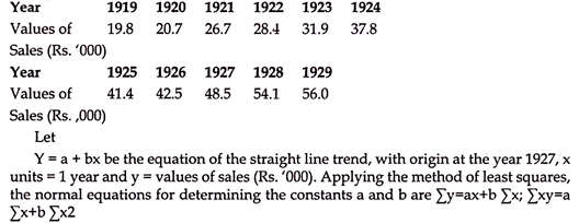
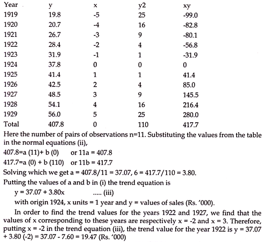
iii. Moving Averages:
This method is used to follow trends in demand data. Here the forecaster simply computes the average value achieved in several recent periods and uses it as a prediction of demand in the next period. This approach presumes that the future will be an average of past achievements.
In moving average method, a series of arithmetic means, known as moving averages are calculated from the given data and these moving averages are used as trend values. This method is very simple and needs no complicated mathematical calculations. A disadvantage of this method is that a few trend values at the beginning and at the end of the series cannot be obtained. The mechanics of this technique can best be illustrated by example.
Illustration:
Assuming a four yearly cycle, calculate the trend by the method of moving averages from the following data relating to the production of tea in India –
iv. Barometric or Leading Indictor Method:
If it is possible to isolate sets of time series which exhibited a close correlation of their movements over time and if one or more of these time series normally led the time series in which the forecaster has interest, then this leading series could be used as a predictor or barometer for short-term changes in the series of interest.
Economic indicators may be classified as leading, coincident or lagging series. The leading series are data on the variables which move up or down ahead of some other series, the coincident series move along with some other series and the lagging series move up or down behind some other series.
The bank rate is the leading interest rate, the rates at which commercial banks accept deposits and lend to private sector are coincident series and the rates at which private money lenders accept deposits and lend to individuals are lagging series.
v. Simultaneous Equations Method:
The simultaneous equations method is a highly sophisticated statistical technique of forecasting. This is also called the complete system approach of forecasting and involves the formulation of a complete model which can explain the behaviours of all the variables which the company can control. The number of equations in such a model equals the number of variables and the model is solved.
vi. Econometric Model Building:
Econometrics may be defined as the application of economic methodology to decision-making. Econometrics is a combination of economic theory, statistical analysis and mathematical model building in order to explain economic relationships. Here we analyse the relationship between a dependent variable and one or more independent variables.
The relationship can be linear, quadratic, cubic or exponential depending upon the influence exercised by the independent variable over a dependent variable. The main techniques of economics that are used in measuring economic relationships are regression and correlation analysis.
In correlation analysis we are determining the degree of association between two variables while in regression analysis we are concerned with finding the functional relationship between the variables in order to make predictions of a particular variable. The variables that are used in predicting the value of the variable are defined as independent variables. In simple bivariate case one independent and one dependent variable are considered and the form of relationship between the two variables is liner.
The first task of the econometrician is to develop hypothesis regarding the relationship between a set of variables and a certain economic phenomenon. The simplest form of econometric model is the single equation model which is frequently used in empirical demand analysis.
For example, in developing a model to forecast the demand for cars, it might be assumed that the number of cars demanded (Qa) is a function of price (P), disposable per capita income (Yd) and advertising expenditures (Ae). If these relationships are linear, an equation can be written as –
Qd = b0 + b1 P + b2 Yd + b3 Ae + ԑ
b0, b1, b2, b3, b4 are parameters to be estimated. Parameter is assumed to be negative while b2, b3, b4 are positive. The above equation shows not only which independent variables explain values of dependent variable but also the form of the relationship between each independent variable and dependent variable.
For example (P) has a negative impact on quantity demanded (Qd) while other independent variables are expected to have positive impact on motor car sales? The term ‘ԑ’ or stochastic variable is included in the model to represent deviations of the observed value from the theoretical value.
If there were no errors then econometric models is that they attempt to explain the economic phenomenon being forecast. Since management is able to manipulate some of the independent variables embodied in this model, econometric models enable management to assess quantitatively the impact of changes in its policies. Moreover, econometric models not only predict the direction of change in an economic series, but also the magnitude of that change.
vii. Forecasting with Input-Output Analysis:
One of the most sophisticated forecasting methods which has been developed is based on Leontief’s input- output model of the economy. Input-output analysis enables the forecaster to trace the effects of an increase in demand for one product through other industries. An increase in demand for motor cars will first lead to an increase in the output of the auto industry.
This in turn will lead to an increase in the demand for steel, tyres, glass, etc. In addition, there will be secondary impacts as the increase in the demand for steel, for example, requires an increase in the production of iron ore which are used to make steel. There may be an increase in the demand for machinery as a result of steel demand and so on. Through input- output analysis the forecaster traces all inter-industry effects which occur as a result of the initial increase in the demand for motor cars.
Input-output analysis has been used in a variety of applications from forecasting sales for an individual firm to evaluating the impacts of major economic programmes. The major contribution of input-output analysis is that it facilitates a detailed tracing and measurement of the effects of all the demands on the output of each industry influenced by an initial change in some final demand.
viii. Computer Assisted Forecasting:
These days’ computers are frequently used for demand forecasting because they are very fast and can make predictions from masses of figures. The computers are programmed to compare predictions generated by alternative methods and keep track of forecasting errors.
Demand Forecasting – Factors involved in Demand Forecasting
The following six factors are involved in demand forecasting:
1. Forecasting may be undertaken at four different levels — international level, macro-level, industry level and firm level. These have already been explained.
2. Forecasting may be general or specific. The firm may find a general forecast about its sales useful. Again sales forecast can be made for specific products or for specific areas of sales.
3. Methods and problems of forecasting are different for new products from established products. For established products past trends are known and can guide future performance.
4. While forecasting, the nature of the commodity should be considered. Commodities are either producers’ goods or consumers’ goods and the pattern of demand is different for different types of goods.
5. Special factors peculiar to the product and the market must be taken into consideration. The nature of the competition in the market as well as the sociological and ecological aspects should not be ignored.
Forecasting the Demand for New Products:
Methods of forecasting demand for new products are quite different from the demand for existing products. For new products an intensive study of the characteristics of the products provides a guide to projections of demand. Forecasting techniques have to be tailored to the particular product.
Joel Dean has suggested the following approaches for forecasting the demand for new products:
Demand for the new product should be projected as an outgrowth and evolution of an existing old product. For example, it may be assumed that colour TV picks up where black and white off. This approach is useful only when the new product is so close to being merely an improvement of an existing product that its demand can be very much a projection of the potential development of the existing product.
According to this approach, the new product is treated as a substitute for some existing product or service. For example, linoleum as a substitute for carpets or polythene bags for cloth bags or ball pens for fountain pens. This approach is very useful if it is used scientifically. Since most of the new products are generally substitutes for old products, they are an improvement on the existing ones.
According to this approach the rate of growth and the ultimate level of demand for the new product can be estimated on the basis of the pattern of growth of established products. For instance, analyse the growth curves of all existing consumer durables and try to establish an empirical law of market development applicable to a new product, say, a TV set.
According to this approach, demand for new product is estimated by making direct enquiries from the final purchasers. Such enquiry may be confined to a sample and the results blown up for the whole population.
Opinion polling or survey of buyers’ intentions as revealed by personal interviews has been widely used to explore the demand for new products. The technique for surveying the intentions of buyers as revealed by personal interviews has been successfully used by many companies to explore the potential demand for a new product.
But this method encounters problems of sampling, probing real intentions and conveying the complexity of multiple alternative choices, even for established products. For new products these problems become more complicated.
According to this method, consumers are approached indirectly. Specialized dealers are contacted because they have an intimate ‘feel’ of the consumers. Dealers’ opinions who are supposedly informed about consumer’s needs are solicited. This in an indirect approach. This approach is quite easy but hard to quantify.
However, bias on the part of dealers cannot be entirely ruled out. It is necessary to guard against undue enthusiasm of some dealers and undue pessimisms of some others. A check on these can be made by seeking corroboration from others in the fields as also by tallying with the forecasts arrived at through other methods.
According to this approach, the new product is offered for sale in a sample market and from this the total demand is estimated for a fully developed market. But the problem of this approach is to identify the sample market. If Calcutta or Mumbai or Delhi is selected as a sample market the characteristic features of such markets are different from those of small towns. Again, if we select Darjeeling or Shimla, the sales would be influenced by the size of the floating tourist population. So an inadvertent experiment without any regard to the peculiarities of the market may result in a huge loss.
Demand Forecasting – Evaluation of Demand Forecasting
It is essential for the firm to appraise and evaluate from time to time its overall demand forecasting system as well as the specific demand forecasting methods and techniques employed by it. When the’ forecasts’ and’ actuals’ come close to each other, it can generally be assumed that the forecasting system is reliable. Likewise, when the ‘forecasts’ and ‘actuals’ differ significant’, it can be assumed that the forecasting system needs improvement.
Such a comparison is feasible only after the details of ‘actual demand’ become available and accordingly, Yet, it has considerable value and utility .If, in addition, d continuous evaluation of the system is also made, it will serve more than a mere post-mortem purpose. With such an ongoing evaluation, refinements of the forecast can be made as one goes along the forecast period;
Evaluation of the forecasting system is essential from another angle as well. Only with an evaluation, it is possible to ascertain which assumptions in the forecasting exercise went wrong and to what extent and why. And such a fact-finding job is a must if the firm wants to improve its forecasting in future.
The variance between ‘forecasts’ and ‘actual’ can occur due to several reasons, like an error in the basic assumptions, an error in the choice of the forecasting method, data deficiency, or computation defects. In some cases it is also possible that an entirely new set of environmental factors has entered the scene and caused the variance. The firm should clearly pinpoint and thoroughly analyse the causes for the variance and improve the forecasting system.
Since all forecasts rest primarily on facts and judgment, the right way to improve the reliability of the forecast is by optimising the use of facts/ data and by improving the quality of judgment. The accuracy of forecasts would improve with improvements – the database.
Demand Forecasts Must be Broken Down Over Smaller Territories and Shorter Time Spans:
For the demand forecasts to be meaningful and useful to those who operate the marketing system at different levels, they must be broken down over smaller territories and shorter time spans. It is natural for any firm to work out in the first instance, the forecast for its total marketing territory -i.e., for the corporation as a whole and for the year as a whole.
This forecast has to be split up over the marketing regions and areas of the consumer and ultimately over each demand territory of the consumer. If the forecast stops with the corporate level, it can only serve as a paper plan; it will not have any meaning or use for those running the marketing system at different levels; to the individual demand man who is working in his demand territory in a remote corner of the country, a national level or regional level estimate of consumer demand can only appear as a formidable number; the estimate of demand and demand in his territory alone can serve him as an intimate pathfinder.
Again, it is not enough if the forecasts are broken down into smaller geographical territories. They must be broken down over shorter time spans as well. Demand forecasts must be worked out for each season, each quarter, each month and each fortnight.
The Linkage between Demand Forecasts and Demand Targets:
The consumer’s demand targets emanate from the demand forecasts. But the demand targets need not be the same as the demand forecasts. The firm may consciously decide for one reason or the other, to be content with a lower level of demand, compared with what it had forecast as the possible level.
For example, the firm may be highly profit-conscious and therefore settle down to the relatively more profitable segments of the market instead of the entire market. 01, it might happen that at the given point of time, the firm lacks the financial and other resources necessary for realising the forecasted demand.
The Linkage between Demand Forecasts and Demand Budgets:
The demand forecasting process and the budgeting process are closely interlinked. In fact, demand forecasting becomes useful only when it is properly integrated into the budgeting.
Demand Forecasting – Qualitative and Quantitative Methods (With Examples)
In the business community, the term forecasting is typically associated with figures; the annual sales forecast is an example. In the social sciences, however, forecasts are frequently produced in a qualitative, verbal form. Both of these are valid, and both offer useful insights.
In general, the qualitative forecasts come into their own in the long term (in strategic and macro forecasting). In these cases the process may also sometimes be described as technological forecasting because this is the discipline in which many of the techniques were first developed. The short-term (tactical and micro) forecasts are usually more quantitative.
The following subsections will examine the qualitative techniques, which are mainly used to describe the longer term. Most sound policy making looks first at the longer term (for its strategy) before examining the shorter term in more detail (for its tactics). We shall extend this principle to forecasting, as it helps put the processes into context.
1. Qualitative Methods:
Qualitative methods describe in words what will happen and the impact that it will bring about. In some cases, this may include significant amounts of statistics, but the context will differ from that of the more normal, numerical quantitative forecasts based on trends.
Qualitative forecasts can be compiled from several sources:
(i) Individual or Expert Opinion:
In practice, most forecasts are prepared by an individual. In a small company it may be the owner and in a larger organization it may be the marketing manager. In the largest of all it may be the brand manager or even the manager of the forecasting department. The individual forecast is inevitably a personal judgment, an opinion often based on experience and industry rules of thumb.
Sales force forecasts are normally viewed as quantitative, because they typically result from forecast sales figures, which may in turn be derived from customers’ forecasts. They are then aggregated to give the total forecast. In reality, they fundamentally incorporate the qualitative judgment of each salesperson despite their apparent numerical accuracy.
One problem with this technique is that it is often used in conjunction with commission systems, where the sales representative, in submitting his or her forecast, is very aware that this will be used as the basis for the following year’s targets and hence his or her income. The process becomes not one of forecasting but one of negotiating targets. This is a poor basis for unbiased forecasts. A more advanced, and time-consuming, approach is to survey all customers to record their buying intentions for the coming year.
An important but rarely used input is the forecasts of the large customers themselves. For example, if you are selling steel to the car industry, you need to understand how that industry is forecasting its own future. The account planning process is an ideal mechanism for this invaluable input.
(ii) Expert Panel Method:
This is the first of the formal ways of applying scientific method to individual opinion. It involves bringing together a panel of experts (business consultants, academic researchers, or corporate executives) to pool their individual forecasts. The individual forecasts may be based on various insights ranging from the respective experts’ time-honed personal experiences in industry to econometric analyses. Then, having confirmed (or at least discussed) their individual cases, a corporate forecast “emerges” and is agreed upon.
As the quality of the forecast depends on the quality of the participants, the panel should consist of the best possible team of relevant experts—both from within the organization and from outside it. As with the jury system, such a panel does seem to determine which really are the best forecasts, particularly when the members of the panel also must implement these forecasts. In general, however, the uncertainty associated with future events is underestimated by others who later review these forecasts. The participants in the forecasting usually recognize all too well the limitations of this method.
One type of expertise is provided by the experts who write various predictions in the Old Farmer’s Almanac. Recently a number of these almanacs predicted huge snowfalls for the winter of 1995. As a result, pre winter sales of salt were up 42 percent from the previous year, snowmobile sales increased 46 percent, snow- blower sales rose 120 percent, and employment at one snowplow maker had to be tripled to keep up with demand. Ironically, however, the huge snowfalls failed to materialize!
Another type of expert panel method is the Delphi technique, originally developed at the Rand Corporation. In this case the (anonymous) experts are quite deliberately not brought together, so as to avoid any bandwagon effect. Instead, a general questionnaire is circulated to the team, asking only for predictions of major changes.
The collected replies, including, for example, predictions of technological changes, are then distributed to the team together with a questionnaire that asks more pointed questions, such as predicting dates for the introduction of new technology or forecasting its impact on the organization. Successive rounds of questioning become increasingly specific, until a sufficiently detailed picture is obtained.
Dawn Jarisch, group company purchasing manager for BICC Cables, recently won a highly coveted Modern Distribution Management (formerly Supply Management) magazine’s Idea of the Year award in the United Kingdom for developing a new technique incorporating elements of the Delphi method—a form of structured brainstorming based on collation and analysis of expert opinion.
She worked in a small central team to devise and promote an alternative technique to produce price predictions for materials budgets. Its iterative approach canvassed and distilled internal opinion—supplemented where necessary by industry and macroeconomic forecasts—to produce minimum and maximum predictions and a reliable mean.
A variation on the use of expert opinion is role playing or simulation, in which the experts involved attempt to deduce how they might react in the equivalent real-life situations. This is an expensive approach that is little used.
Still another technique is to ask experts about events similar to the issue under investigation in order to formulate an analogy. For instance, this analogy may come from history, from another field, or from another country. If the analogy matches the parameters involved it can offer a useful insight into the processes at work. For example, how China’s socialistic regime might crumble in the future can be conjectured by experts who examine how the Soviet regime collapsed.
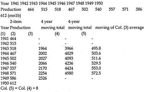
(iii) Technological Forecasting:
This series of techniques is associated with plotting very long-term trends and, in particular, with changes in technology. The estimates are typically based on a plot of the previous changes over time (a growth curve), showing, for example, the increasing performance or decreasing cost.
One classic example is shown in Figure 6.3. The brightness of the lamp, measured by lumens watt per energy unit, has increased at an exponential rate as a result of significant inventions over the years. Using this historical line, one can forecast the brightness of a yet-to-be-developed lamp in the future with a reasonable level of certainty.
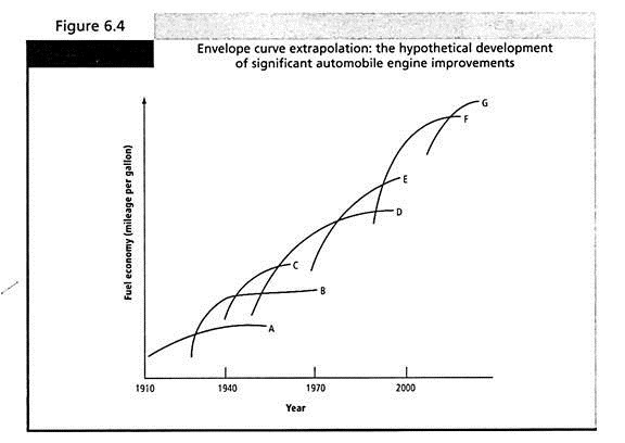
Another related technological forecasting method is an envelope curve extrapolation. An envelope curve expects technology to develop by quantum leaps, with new techniques gradually being improved until they reach the ceiling of their performance, at which point they are then overtaken by the next development. The hypothetical graph in Figure 6.4 illustrates this approach in the context where it is usually deployed.
(iv) Decision Tree:
One aid to qualitative forecasting is the use of tree structures. The main factors affecting the organization’s environment, for example, are plotted, and the possible alternatives or decisions (hence the name decision trees) are shown at each stage, branching at each level like a tree.
At the end of this process, all of the various possible contributions, or at least all that the forecaster chooses to take into account, will have been documented, including some that might not otherwise have been considered. This is the main value of the technique, although an obvious problem is dealing with the sheer number of alternatives that becomes apparent.
One application of the decision tree approach is to apply probabilities to each of the decisions. Bayes’s Theorem offers a simple formula for dealing with conditional probability.
The resulting probabilities of all the possible outcomes can then be calculated. This process can be taken even further by calculating the composite payoffs (the product of the calculated value of the outcome multiplied by the probability) for each alternative.
With computing power now easily available, these quantified outputs can help give a good measure of the optimum outcomes, as long as, once more, it is recognized that all the input factors are opinions rather than hard facts. The wise forecaster also tries to understand how the various elements interact. The same payoff may be achieved by low risks on low-return activities or high risks on high returns—and most organizations would probably favor the former.
(v) Scenario:
This method combines the input from various forecasting techniques, especially the expert opinion and Delphi methods, to give an integrated view. Regrettably, it is rarely used because it requires some significant effort. The fleshing out of the bare-bones forecasts and their integration into a whole scenario means, on the one hand, that it is easier to detect incompatibilities between the various forecasts. On the other hand, it allows extrapolations of these individual forecasts to cover all the activities of the organization.
The identification of crucial trend variables and the degree of their variation is of major importance in scenario building. Frequently, key experts are used to gain information about potential variations and the viability of certain scenarios.
A wide variety of scenarios must be built to expose corporate executives to multiple potential occurrences. Ideally, even far-fetched factors deserve some consideration to build scenarios ranging from the best to the worst. A scenario for Union Carbide Corporation, for example, could have included the possibility of a disaster such as occurred in Bhopal, India.
Similarly, oil companies need to work with scenarios that factor in dramatic shifts in the supply situation, such as those precipitated by regional conflict in the Middle East. They should consider major alterations in the demand picture, due to, say, technological developments or government policies.
Scenario builders also need to recognize the unpredictability of some factors. To simply extrapolate from currently existing situations is insufficient. Frequently, unexpected factors may enter the picture with significant impact.
For example, despite some prediction about the climatic effects of El Nino and El Nina, insurance companies never expected the level of devastations wrought by hurricanes and tornadoes in the United States due to the cyclical warming and cooling of the tropical water in the Pacific. Finally, given large technological advances, the possibility of “wholesale” obsolescence of current technology must also be considered. For example, quantum leaps in computer development and Internet technology may render obsolete the technological investment of a corporation or even a country.
For scenarios to be useful, management must analyze and respond to them by formulating contingency plans. Such planning will broaden horizons and may ‘prepare management for unexpected situations. Familiarization in turn can result in shorter response times to actual occurrences by honing response capability. The difficulty, of course, is to devise scenarios that are unusual enough to trigger new thinking yet sufficiently realistic to be taken seriously by management.
The development of a marketing decision support system is of major importance to many firms. It aids the ongoing decision process and becomes a vital corporate tool in carrying out the strategic planning task. Only by observing global trends and changes will the firm be able to maintain and increase its competitive position.
Many of the data available are quantitative in nature, but attention must also be paid to qualitative dimensions. Quantitative analysis will continue to improve as the ability to collect, store, analyze, and retrieve data increases through the use of high-speed computers. Nevertheless, qualitative analysis will remain a major component of corporate research and strategic planning.
2. Quantitative Methods:
In general, most quantitative techniques revolve around time-series analysis of historical statistics. They treat the systems involved as a black box. As such, they can only be as reliable as those statistics at best, and hence are best applied to in- house statistics, such as sales figures, where the accuracy (and likely limitation) is better understood.
On the other hand, explanatory models try to set out how these systems work so that the effect of future changes can also be predicted. They are consequently more powerful, but significantly more difficult to build.
Sales trend forecasting is the scientific approach favored by most management, because it is seen to project forward the historical trends that they have already observed. Thus, if sales have increased by 15 percent for each of the previous three years, the assumption is that they will also increase by around 15 percent in the coming year. We have already seen, though, how the fishbone effect may sometimes invalidate these confident assumptions. Also, as the base broadens, growth rates will be more difficult to maintain.
The simplest and most common form of forecasting is handled manually or by using the now omnipresent electronic pocket calculator or personal computer. The processes are still simple mechanized analogues of the manual processes. These forecasts project the trends shown by recent historical sales figures. Again, this is best viewed as a variation of pure judgment.
Although these simple manual techniques have great strengths, they are limited by the subjectivity of their conclusions. The more sophisticated techniques (explained below) have almost as many assumptions built into them but, because these value judgments are not immediately obvious, they tend to be seen (incorrectly) as having inherently greater accuracy. Whether you use manual or more sophisticated techniques, you should be always aware of their limitations and assumptions before making any decision based on your forecast.
(i) Mathematical Techniques:
There are a number of mathematical techniques (some of great complexity) that apparently provide a strong scientific basis.
However, in essence, most of them allow for just four components in any such forecast:
a. Trend:
The ongoing growth (or decline) of the product or service is determined by fitting a straight or, occasionally, a curved line to the historical sales data.
b. Cyclical:
Any wavelike movement over the years reflects, for example, general business trends. The problem in this cyclical case is identifying which (if any) is the true cycle and not just an artifact. It is more difficult still to determine whether the cycle will be repeated again in the future. The decades-long Kondratieff Cycles, which are often discussed in economic theory, are more difficult to observe (if they are present at all) and are consequently more controversial. However, Yoshihiro Kogane offers one succinct analysis of these cycles over the past two centimes.
c. Seasonal:
Many products or services are seasonal with some distinctive fluctuations, usually over a period of a year, that remain rather consistent over time, and this pattern is overlaid on the others.
d. Random Events:
Most sales graphs show unpredictable effects, such as industry disputes, although some (such as planned promotional campaigns) may be predictable to a certain extent.
(ii) Period Actuals and Percentage Changes:
The forecast may simply and, most frequently, continue the trends observed in previous periods. This may be achieved either by calculating the average percentage increase or by drawing the best-possible straight line through the historical figures when plotted on a graph.
There are three related methods of this forecast, using period actuals and percentage changes:
a. Moving Annual Total:
This technique smoothed out short-term fluctuations (especially seasonality) by moving forward the accumulated total for the preceding 12 months. Thus, each new month’s figures are added to the previous (MAT) total, and the comparable figures from a year ago are deducted. The forecast is once more obtained by extending the trend line; this time smoothed by the incorporation of the whole year’s data.
b. Cumulative Totals:
This measure is normally used in the context of control (measuring how cumulative sales are performing against target, for example) rather than as a forecasting tool.
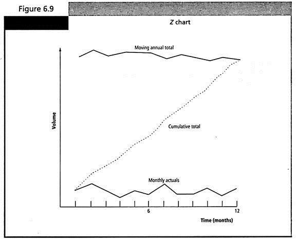
c. Z Charts:
As shown in Figure 6.9, all of these data (for one year) can be neatly combined on one graph, a Z chart. The bottom bar of the Z is made up of the monthly actuals, whereas the top bar is the moving annual total. The diagonal eventually joining them is the cumulative figure (equal to the first month actual at the left and the moving annual total at the end of the year at the right).
(iii) Exponential Smoothing:
This is a simple but useful mathematical technique that allows greater weight to be given to recent periods. For example, instead of the average trend over the whole of the last year being calculated, the sales data for each of the months is given a weighting, depending on how recent that month was.
In a manner somewhat akin to the moving annual total, it takes the previous figure, in this case the moving forecast, and adds on the latest actual sales figure. However, it does this in a fixed proportion that is chosen to reflect the weighting to be given to the latest period.
The general formula is:
Ft+1 = Ft + aEt
Where Ft+1 is the new forecast, Ft is the previous one, and Et is the deviation (or error) of the actual new performance recorded against the previous period forecast; a is the weighting to be given to the most recent events. In this simple form, exponential smoothing will not allow for seasonality, although more advanced (but less easily understood) versions can do this.
(iv) Advanced Time-Series Analyses and Models:
In general, to account for the variations due to seasonal trends as well as for those due to long-term trends, more sophisticated calculations, such as mathematical modeling, are needed. Models are merely more complex equations.
General time-series models can be built by arithmetically removing a steady overall trend (the straight line showing the long-term average increase) and by measuring deviations from it to give the underlying, average, seasonal pattern. Models can also be built by visual inspection (as the Z chart was).
Auto-Regressive Moving Average (ARMA) techniques are the most sophisticated of the simple time-series methods. They filter out the various effects of cycle and seasonality to detect the underlying growth. The most commonly reported method is Box-Jenkins. Although widely reported in the literature, these advanced techniques are relatively little used in practice.
(v) Multiple Regression Analysis:
At the more advanced level, computers are extensively used to conduct regression analyses on the elements of the model. Regression analysis determines the strengths of the relationship of one variable with other variables involved.
In simple regression, a linear, straight line relationship of the form is assumed –
y = a + bx
Where a and b are the constants (to be found). Regression analysis is designed to explain or to predict a criterion variable (y), based on a predictor variable (x). This does not even require the use of a computer, but such simple relationships are rare.
Usually a number of predictor variables are involved for prediction, so that multiple regression analyses become necessary. Then computer programs are used to determine statistically from the historical data and the changes in the various variables what the likelihood is of each of the predictor variables having an impact on the criterion variable. The parameters of the model and the overall probabilities of each outcome can then be determined.
For example, in order to predict annual automobile sales for first-time buyers in the United States, various factors can be considered in the regression model, as follows:
Annual automobile sales = a + b1x (number of college graduates) + b2x (interest rate) + b3x (unemployment rate) + …
(vi) Econometric Models:
Very large econometric models, which simulate the workings of national economies, can contain hundreds of factors spread across dozens of linked equations and can require large amounts of computing power. Unfortunately, as a result, they are barely understandable even to those running them. This econometric model shows how the various factors in boxes will affect, and be affected by, other factors.
Arrows represent causal effects. However, these models are often seen as almost infallible largely due to their immense complexity. This is despite, or possibly because of, the general ignorance of many of those involved. Changes in government policy, for instance, are often run against the models of the national economy to see what will happen rather than what might happen.
Econometric-type models are also being used to help manage the new- product introduction strategy. Compaq employed complex simulation software to plan the timing of the switch from 486-based to Pentium-based computers. The program was designed to model the latest trends in consumer demand, pricing, and dealer inventories.
Based on the model, Compaq decided to wait several months after their competitors to introduce its own Pentium machines. The decision preserved the value of Compaq’s 486 inventory and led to a 61 percent increase in fourth-quarter 1994 earnings, boosting profits by $50 million. However, as initially developed by Dell Computer, the “build-to-order” model of product development and sales fulfillment has started replacing the “build-to-forecast” model, and the traditional role of sales forecasting has begun waning into the 21st century.
(vii) Leading Indicators:
It may be possible to establish that certain factors are leading indicators in that they provide advance warning of future trends. For example, it may be that suppliers of pop CDs should study the birthrate statistics to see how their total teenage market may vary in future years.
In the United States, there are a range of useful published statistics that are widely used as indicators – U.S. Durable Goods Orders, movements of which may indicate the general economy some six months ahead; Housing Starts, perhaps 10 to 12 months ahead; and Interest Rates on Three-Month Certificates of Deposit, which is supposed to give an indication for 18 months ahead.
One of the most useful—and most obvious in its workings—is the leading indicator offered by the Conference Board’s Consumer Confidence Index. Other useful leading indicators include Stock Prices, Corporate Bond Yield, Industrial Materials Prices, Business Failures, Money Supply, Unemployment Rate, Producer Price Index, Consumer Price Index, and Business Inventories.
In forecasting the market conditions of foreign countries, marketers can use a country’s leading indicators similar to the ones available in the United States and also the country’s trade balance and exchange rates as international leading indicators. A country’s continued trade deficit usually indicates either that its government will tighten its fiscal and monetary policy, thereby reducing domestic consumption, or that its currency will depreciate, thereby making imported products more expensive.
Either way, a country’s trade deficit will portend its reduced purchasing power. To predict a foreign country’s purchasing power, marketers may simply look at 180-day forward exchange rates in the Foreign Exchange Rate section of the Wall Street Journal. If forward exchange rates seem to be depreciating fast, then it generally indicates a pending reduction in purchasing power.
(viii) Game Theory:
Defined as “the study of rational behavior in situations involving interdependence,” game theory has recently received enhanced notoriety on two fronts. First, in 1994 three game theorists received the Nobel Prize in economics, and second, game theory was used extensively by the U.S. Federal Communications Commission to assist in auctioning off the wavelengths necessary to support pagers and pocket telephones.
Before game theory, most economic models assumed that firms were basically acting in a vacuum. The actions of one firm were not assumed to impact the actions of other firms. That economic assumption is true as long as markets are perfectly competitive or where pure monopolies exist. Game theory allows for corporate action, competitor reaction, corporate action, and on and on. Unfortunately, game theory is difficult to use because of its complex mathematics. However, it is now being taught at many leading MBA programs, which means that it will be increasingly used in coming years.
3. Spreadsheets:
In the context of forecasting and planning, probably the most useful tool that personal computers provide is the now ubiquitous spreadsheet. Despite its apparent simplicity, even this tool is often misused by managers, who see it merely as a more sophisticated calculator. In the present context, however, it has a number of powerful contributions to make.
One important use of spreadsheets is the mechanization of routine budgets. The whole planning cycle is bedeviled by the grind of cranking out large numbers of routine figures. Many, if not most, of these are derived from other figures and ultimately lead back to a relatively few indirect variables entered into the model. Once these linkages are entered onto a spreadsheet, the planning cycle becomes much easier. However, there are dangers even in this seemingly straightforward approach, not least of which is that spreadsheets lock into the model all the existing assumptions about the relationships.
There are two solutions to this dilemma:
(i) Clear structure – The spreadsheet should be designed in such a way that the linkages (and hence the assumptions) are obvious and are easy to change.
(ii) Process of challenge – Some of the time saved by using the spreadsheet should be used routinely to challenge the assumptions to ensure that they are still valid.
Perhaps the most important use of spreadsheets is to question these assumptions. The ease with which calculations can be repeated with different assumptions means that the marketing manager can try out all of the different alternatives. This iterative process is called sensitivity analysis, and can then be used to fine-tune, or optimize, the key parameters.
Although widely used spreadsheets, such as Microsoft Excel and Lotus 1-2-3, remain useful, spreadsheet add-ons, such as Palisade Corporation’s @ Risk, could provide more powerful analytical tools for decision making.
Modeling:
Spreadsheets can be used to build crude models. For example, a model of the seasonal, trend, and cyclic components of sales figures (as well as the impact of promotions) can be created from eyeballing the graphs of historical sales and fine-tuning the resulting model parameters until the results obtained most closely fit the historical results. This process may be time consuming and lacking the elegance of the advanced techniques, but it may also produce results that are almost as good (and more easily understood).
Alternatives to Forecasting:
There are a number of alternatives to forecasting that can also help reduce risk— including that due to poor forecasting—if not the need for some form of formal planning.
(i) Insurance – Future movements in exchange rates, for instance, may be covered by hedges on the financial futures market.
(ii) Portfolios – Risk can be spread by entering a number of different markets or introducing a number of different products that are unlikely to face the same economic downturns or competition.
(iii) Flexibility – The Japanese in particular have developed means for coping rapidly with unexpected changes.
Flexibility:
Of the alternatives listed above, flexibility is emerging as the most important. This is most evident in the development, mainly by Japanese corporations, of flexible manufacturing and dramatically reduced development lead times for high-tech goods. But similarly accelerated time scales can be even more easily applied where technological development is less demanding and the promotional activities need to be changed rapidly.
This approach, although not superseding others, simply requires that once change has been detected the reaction time should be so fast that the response may be implemented before the change reaches a significant level. More importantly, the response time should be faster than that of competitors who might otherwise be able to take advantage of the change. However, such an approach requires a very sophisticated early detection method for environmental change.
Factors Limiting Forecasts:
Spyros Makridakis sums up the most likely errors and biases in forecasting. The most frequent mistake in practice is sometimes called the hockey stick effect When actual results fail to live up to optimistic forecasts, the starting point of the new forecast is changed to allow for this, but the slope of the forecast line remains (still optimistically) unchanged. Nobody in the forecasting process asks why the forecast was missed—and nobody learns from experience.
Perhaps the greatest practical limitation on forecasting, however, is its incorrect use due to a lack of knowledge by managers. A survey by McHugh and Sparkes came to the now classic conclusion that
… despite the need and the fact that the results of past forecasting performance reveal a high level of inaccuracy it seems that not only do naive techniques dominate (representing 90% of techniques currently utilized) but also very few respondents are taking steps to improve the situation … The main problem seemed to be that there was a total lack of specific techniques, particularly the Delphi method, cross- impact analysis and Box-Jenkins and in the case of causal model-building, regression and correlation analysis, the problem seems to be a lack of working experience of the particular techniques.
In fact, users prefer simple, intuitive, easy-to-use, easy-to-comprehend methods. It is these factors, rather than accuracy, that are ultimately desired, which determine when and how forecasting is used. The practical effect of all these limitations often results in a forecasting phenomenon, usually relating to long-range forecasting, known as the cliff. In essence, management uses forecasting for a period of time (albeit often without fully understanding why and how it should be carried out) until the point at which problems arise. All formal forecasting is then summarily stopped, as if dropped off a cliff.